A Practical Introduction to Factor Analysis: Exploratory Factor Analysis |
您所在的位置:网站首页 › common method variance › A Practical Introduction to Factor Analysis: Exploratory Factor Analysis |
A Practical Introduction to Factor Analysis: Exploratory Factor Analysis
|
Purpose
This seminar is the first part of a two-part seminar that introduces central concepts in factor analysis. Part 1 focuses on exploratory factor analysis (EFA). Although the implementation is in SPSS, the ideas carry over to any software program. Part 2 introduces confirmatory factor analysis (CFA). Please refer to A Practical Introduction to Factor Analysis: Confirmatory Factor Analysis. I. Exploratory Factor Analysis Introduction Motivating example: The SAQ Pearson correlation formula Partitioning the variance in factor analysis Extracting factors principal components analysis common factor analysis principal axis factoring maximum likelihood Rotation methods Simple Structure Orthogonal rotation (Varimax) Oblique (Direct Oblimin) Generating factor scores Back to Launch Page IntroductionSuppose you are conducting a survey and you want to know whether the items in the survey have similar patterns of responses, do these items “hang together” to create a construct? The basic assumption of factor analysis is that for a collection of observed variables there are a set of underlying variables called聽factors (smaller than the observed variables), that can explain the interrelationships among those variables. Let’s say you conduct a survey and collect responses about people’s anxiety about using SPSS. Do all these items actually measure what we call “SPSS Anxiety”?
Let’s proceed with our hypothetical example of the survey which Andy Field terms the SPSS Anxiety Questionnaire. For simplicity, we will use the so-called “SAQ-8” which consists of the first eight items in the SAQ. Click on the preceding hyperlinks to download the SPSS version of both files. The SAQ-8 consists of the following questions: Statistics makes me cry My friends will think I’m stupid for not being able to cope with SPSS Standard deviations excite me I dream that Pearson is attacking me with correlation coefficients I don’t understand statistics I have little experience of computers All computers hate me I have never been good at mathematics Pearson Correlation of the SAQ-8Let’s get the table of correlations in SPSS Analyze – Correlate – Bivariate: Correlations 1 2 3 4 5 6 7 8 1 1 2 -.099** 1 3 -.337** .318** 1 4 .436** -.112** -.380** 1 5 .402** -.119** -.310** .401** 1 6 .217** -.074** -.227** .278** .257** 1 7 .305** -.159** -.382** .409** .339** .514** 1 8 .331** -.050* -.259** .349** .269** .223** .297** 1 **. Correlation is significant at the 0.01 level (2-tailed). *. Correlation is significant at the 0.05 level (2-tailed).From this table we can see that most items have some correlation with each other ranging from \(r=-0.382\) for Items 3 and 7 to \(r=.514\) for Items 6 and 7. Due to relatively high correlations among items, this would be a good candidate for factor analysis. Recall that the goal of factor analysis is to model the interrelationships between items with fewer (latent) variables. These interrelationships can be broken up into multiple components Partitioning the variance in factor analysisSince the goal of factor analysis is to model the interrelationships among items, we focus primarily on the variance and covariance rather than the mean. Factor analysis assumes that variance can be partitioned into two types of variance, common and unique Common variance is the amount of variance that is shared among a set of items. Items that are highly correlated will share a lot of variance. Communality (also called \(h^2\)) is a definition of common variance that ranges between \(0 \) and \(1\). Values closer to 1 suggest that extracted factors explain more of the variance of an individual item. Unique variance is any portion of variance that’s not common. There are two types: Specific variance: is variance that is specific to a particular item (e.g., Item 4 “All computers hate me” may have variance that is attributable to anxiety about computers in addition to anxiety about SPSS). Error variance:聽comes from errors of measurement and basically anything unexplained by common or specific variance (e.g., the person got a call from her babysitter that her two-year old son ate her favorite lipstick).The figure below shows how these concepts are related:
As a data analyst, the goal of a factor analysis is to reduce the number of variables to explain and to interpret the results. This can be accomplished in two steps: factor extraction factor rotationFactor extraction involves making a choice about the type of model as well the number of factors to extract. Factor rotation comes after the factors are extracted, with the goal of achieving聽simple structure聽in order to improve interpretability. Extracting FactorsThere are two approaches to factor extraction which stems from different approaches to variance partitioning: a) principal components analysis and b) common factor analysis. Principal Components AnalysisUnlike factor analysis, principal components analysis or PCA makes the assumption that there is no unique variance, the total variance is equal to common variance. Recall that variance can be partitioned into common and unique variance. If there is no unique variance then common variance takes up total variance (see figure below). Additionally, if the total variance is 1, then the common variance is equal to the communality. 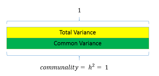 Running a PCA with 8 components in SPSS Running a PCA with 8 components in SPSS
The goal of a PCA is to replicate the correlation matrix using a set of components that are fewer in number and linear combinations of the original set of items. Although the following analysis defeats the purpose of doing a PCA we will begin by extracting as many components as possible as a teaching exercise and so that we can decide on the optimal number of components to extract later. First go to Analyze – Dimension Reduction – Factor. Move all the observed variables over the Variables: box to be analyze.
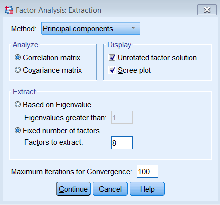
Under Extraction – Method, pick Principal components and make sure to Analyze the Correlation matrix. We also request the Unrotated factor solution and the Scree plot. Under Extract, choose Fixed number of factors, and under Factor to extract enter 8. We also bumped up the Maximum Iterations of Convergence to 100.
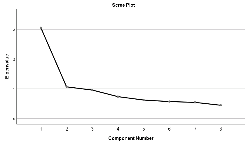
The equivalent SPSS syntax is shown below: FACTOR /VARIABLES q01 q02 q03 q04 q05 q06 q07 q08 /MISSING LISTWISE /ANALYSIS q01 q02 q03 q04 q05 q06 q07 q08 /PRINT INITIAL EXTRACTION /PLOT EIGEN /CRITERIA FACTORS(8) ITERATE(100) /EXTRACTION PC /ROTATION NOROTATE /METHOD=CORRELATION. Eigenvalues and EigenvectorsBefore we get into the SPSS output, let’s understand a few things about eigenvalues and eigenvectors. Eigenvalues represent the total amount of variance that can be explained by a given principal component. 聽They can be positive or negative in theory, but in practice they explain variance which is always positive. If eigenvalues are greater than zero, then it’s a good sign. Since variance cannot be negative, negative eigenvalues imply the model is ill-conditioned. Eigenvalues close to zero imply there is item multicollinearity, since all the variance can be taken up by the first component.Eigenvalues are also the sum of squared component loadings across all items for each component, which represent the amount of variance in each item that can be explained by the principal component. Eigenvectors represent a weight for each eigenvalue. The eigenvector times the square root of the eigenvalue gives the component loadings聽which can be interpreted as the correlation of each item with the principal component. For this particular PCA of the SAQ-8, the 聽eigenvector associated with Item 1 on the first component is \(0.377\), and the eigenvalue of Item 1 is \(3.057\). We can calculate the first component as $$(0.377)\sqrt{3.057}= 0.659.$$ In this case, we can say that the correlation of the first item with the first component is \(0.659\). Let’s now move on to the component matrix. Component MatrixThe components can be interpreted as the correlation of each item with the component.聽Each item has a loading corresponding to each of the 8 components. For example, Item 1 is correlated \(0.659\) with the first component, \(0.136\) with the second component and \(-0.398\) with the third, and so on. The square of each loading represents the proportion of variance (think of it as an \(R^2\) statistic) explained by a particular component. For Item 1, \((0.659)^2=0.434\) or \(43.4\%\) of its variance is explained by the first component. Subsequently, \((0.136)^2 = 0.018\) or \(1.8\%\) of the variance in Item 1 is explained by the second component. The total variance explained by both components is thus \(43.4\%+1.8\%=45.2\%\). If you keep going on adding the squared loadings cumulatively down the components, you find that it sums to 1 or 100%. This is also known as the communality, and in a PCA the communality for each item is equal to the total variance. Component Matrixa Item Component 1 2 3 4 5 6 7 8 1 0.659 0.136 -0.398 0.160 -0.064 0.568 -0.177 0.068 2 -0.300 0.866 -0.025 0.092 -0.290 -0.170 -0.193 -0.001 3 -0.653 0.409 0.081 0.064 0.410 0.254 0.378 0.142 4 0.720 0.119 -0.192 0.064 -0.288 -0.089 0.563 -0.137 5 0.650 0.096 -0.215 0.460 0.443 -0.326 -0.092 -0.010 6 0.572 0.185 0.675 0.031 0.107 0.176 -0.058 -0.369 7 0.718 0.044 0.453 -0.006 -0.090 -0.051 0.025 0.516 8 0.568 0.267 -0.221 -0.694 0.258 -0.084 -0.043 -0.012 Extraction Method: Principal Component Analysis. a. 8 components extracted.Summing the squared component loadings across the components (columns) gives you the communality estimates for each item, and summing each squared loading down the items (rows) gives you the eigenvalue for each component. For example, to obtain the first eigenvalue we calculate: $$(0.659)^2 + 聽(-.300)^2 – (-0.653)^2 + (0.720)^2 + (0.650)^2 + (0.572)^2 + (0.718)^2 + (0.568)^2 = 3.057$$ You will get eight eigenvalues for eight components, which leads us to the next table. Total Variance Explained in the 8-component PCA Recall that the eigenvalue represents the total amount of variance that can be explained by a given principal component. Starting from the first component, each subsequent component is obtained from partialling out the previous component. Therefore the first component explains the most variance, and the last component explains the least. Looking at the Total Variance Explained table, you will get the total variance explained by each component. For example, Component 1 is \(3.057\), or \((3.057/8)\% = 38.21\%\) of the total variance. Because we extracted the same number of components as the number of items, the Initial Eigenvalues column is the same as the Extraction Sums of Squared Loadings column. Total Variance Explained Component Initial Eigenvalues Extraction Sums of Squared Loadings Total % of Variance Cumulative % Total % of Variance Cumulative % 1 3.057 38.206 38.206 3.057 38.206 38.206 2 1.067 13.336 51.543 1.067 13.336 51.543 3 0.958 11.980 63.523 0.958 11.980 63.523 4 0.736 9.205 72.728 0.736 9.205 72.728 5 0.622 7.770 80.498 0.622 7.770 80.498 6 0.571 7.135 87.632 0.571 7.135 87.632 7 0.543 6.788 94.420 0.543 6.788 94.420 8 0.446 5.580 100.000 0.446 5.580 100.000 Extraction Method: Principal Component Analysis. Choosing the number of components to extractSince the goal of running a PCA is to reduce our set of variables down, it would useful to have a criterion for selecting the optimal number of components that are of course smaller than the total number of items. One criterion is the choose components that have eigenvalues greater than 1. Under the Total Variance Explained table, we see the first two components have an eigenvalue greater than 1. This can be confirmed by the Scree Plot which plots the eigenvalue (total variance explained) by the component number. Recall that we checked the Scree Plot option under Extraction – Display, so the scree plot should be produced automatically.
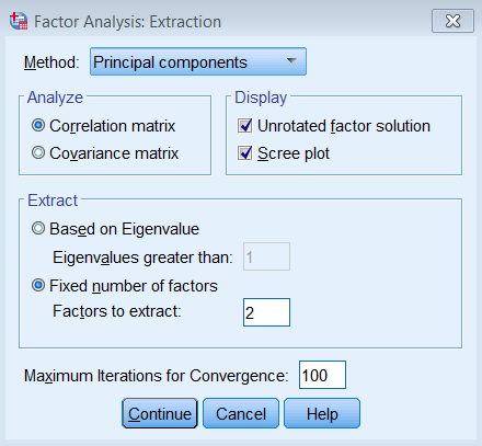
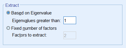
The first component will always have the highest total variance and the last component will always have the least, but where do we see the largest drop? If you look at Component 2, you will see an “elbow” joint. This is the marking point where it’s perhaps not too beneficial to continue further component extraction. There are some conflicting definitions of the interpretation of the scree plot but some say to take the number of components to the left of the the “elbow”. Following this criteria we would pick only one component. A more subjective interpretation of the scree plots suggests that any number of components between 1 and 4 would be plausible and further corroborative evidence would be helpful. Some criteria say that the total variance explained by all components should be between 70% to 80% variance, which in this case would mean about four to five components. The authors of the book say that this may be untenable for social science research where extracted factors usually explain only 50% to 60%. Picking the number of components is a bit of an art and requires input from the whole research team. Let’s suppose we talked to the principal investigator and she believes that the two component solution makes sense for the study, so we will proceed with the analysis. Running a PCA with 2 components in SPSSRunning the two component PCA is just as easy as running the 8 component solution. The only difference is under Fixed number of factors – Factors to extract you enter 2.
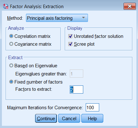
We will focus the differences in the output between the eight and two-component solution. Under Total Variance Explained, we see that the Initial Eigenvalues no longer equals the Extraction Sums of Squared Loadings. The main difference is that there are only two rows of eigenvalues, and the cumulative percent variance goes up to \(51.54\%\). Total Variance Explained Component Initial Eigenvalues Extraction Sums of Squared Loadings Total % of Variance Cumulative % Total % of Variance Cumulative % 1 3.057 38.206 38.206 3.057 38.206 38.206 2 1.067 13.336 51.543 1.067 13.336 51.543 3 0.958 11.980 63.523 4 0.736 9.205 72.728 5 0.622 7.770 80.498 6 0.571 7.135 87.632 7 0.543 6.788 94.420 8 0.446 5.580 100.000 Extraction Method: Principal Component Analysis.Similarly, you will see that the Component Matrix has the same loadings as the eight-component solution but instead of eight columns it’s now two columns. Component Matrixa Item Component 1 2 1 0.659 0.136 2 -0.300 0.866 3 -0.653 0.409 4 0.720 0.119 5 0.650 0.096 6 0.572 0.185 7 0.718 0.044 8 0.568 0.267 Extraction Method: Principal Component Analysis. a. 2 components extracted.Again, we interpret Item 1 as having a correlation of 0.659 with Component 1. From glancing at the solution, we see that Item 4 has the highest correlation with Component 1 and Item 2 the lowest. Similarly, we see that Item 2 has the highest correlation with Component 2 and Item 7 the lowest. Quick check:True or False The elements of the Component Matrix are correlations of the item with each component. The sum of the squared eigenvalues is the proportion of variance under Total Variance Explained. The Component Matrix can be thought of as correlations and the Total Variance Explained table can be thought of as \(R^2\).1.T, 2.F (sum of squared loadings), 3. T Communalities of the 2-component PCAThe communality is the sum of the squared component loadings up to the number of components you extract. In the SPSS output you will see a table of communalities. Communalities Initial Extraction 1 1.000 0.453 2 1.000 0.840 3 1.000 0.594 4 1.000 0.532 5 1.000 0.431 6 1.000 0.361 7 1.000 0.517 8 1.000 0.394 Extraction Method: Principal Component Analysis.Since PCA is an iterative estimation process, it starts with 1 as an initial estimate of the communality (since this is the total variance across all 8 components), and then proceeds with the analysis until a final communality extracted. Notice that the Extraction column is smaller Initial column because we only extracted two components. As an exercise, let’s manually calculate the first communality from the Component Matrix. The first ordered pair is \((0.659,0.136)\) which represents the correlation of the first item with Component 1 and Component 2. Recall that squaring the loadings and summing down the components (columns) gives us the communality: $$h^2_1 = (0.659)^2 + (0.136)^2 = 0.453$$ Going back to the Communalities table, if you sum down all 8 items (rows) of the Extraction column, you get \(4.123\). If you go back to the Total Variance Explained table and summed the first two eigenvalues you also get \(3.057+1.067=4.124\). Is that surprising? Basically it’s saying that the summing the communalities across all items is the same as summing the eigenvalues across all components. Quiz1. In a PCA, when would the communality for the Initial column be equal to the Extraction column? Answer: When you run an 8-component PCA. True or False The eigenvalue represents the communality for each item. For a single component, the sum of squared component loadings across all items represents the eigenvalue for that component. The sum of eigenvalues for all the components is the total variance. The sum of the communalities down the components is equal to the sum of eigenvalues down the items.Answers: 1. F, the eigenvalue is the total communality across all items for a single component, 2. T, 3. T, 4. F (you can only sum communalities across items, and sum eigenvalues across components, but if you do that they are equal). Common Factor AnalysisThe partitioning of variance differentiates a principal components analysis from what we call common factor analysis. Both methods try to reduce the dimensionality of the dataset down to fewer unobserved variables, but whereas PCA assumes that there common variances takes up all of total variance, common factor analysis assumes that total variance can be partitioned into common and unique variance. It is usually more reasonable to assume that you have not measured your set of items perfectly. The unobserved or latent variable that makes up common variance is called a factor, hence the name factor analysis. The other main difference between PCA and factor analysis lies in the goal of your analysis. If your goal is to simply reduce your variable list down into a linear combination of smaller components then PCA is the way to go. However, if you believe there is some latent construct that defines the interrelationship among items, then factor analysis may be more appropriate. In this case, we assume that there is a construct called SPSS Anxiety that explains why you see a correlation among all the items on the SAQ-8, we acknowledge however that SPSS Anxiety cannot explain all the shared variance among items in the SAQ, so we model the unique variance as well. Based on the results of the PCA, we will start with a two factor extraction. Running a Common Factor Analysis with 2 factors in SPSSTo run a factor analysis, use the same steps as running a PCA (Analyze – Dimension Reduction – Factor) except under Method choose Principal axis factoring. Note that we continue to set Maximum Iterations for Convergence at 100 and we will see why later.
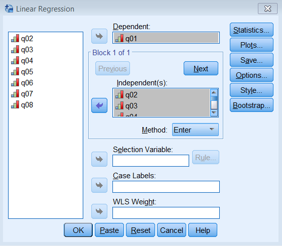
Pasting the syntax into the SPSS Syntax Editor we get: FACTOR /VARIABLES q01 q02 q03 q04 q05 q06 q07 q08 /MISSING LISTWISE /ANALYSIS q01 q02 q03 q04 q05 q06 q07 q08 /PRINT INITIAL EXTRACTION /PLOT EIGEN /CRITERIA FACTORS(2) ITERATE(100) /EXTRACTION PAF /ROTATION NOROTATE /METHOD=CORRELATION.Note the main difference is under /EXTRACTION we list PAF for Principal Axis Factoring instead of PC for Principal Components. We will get three tables of output, Communalities, Total Variance Explained and Factor Matrix. Let’s go over each of these and compare them to the PCA output. Communalities of the 2-factor PAF Communalities Item Initial Extraction 1 0.293 0.437 2 0.106 0.052 3 0.298 0.319 4 0.344 0.460 5 0.263 0.344 6 0.277 0.309 7 0.393 0.851 8 0.192 0.236 Extraction Method: Principal Axis Factoring.The most striking difference between this communalities table and the one from the PCA is that the initial extraction is no longer one. Recall that for a PCA, we assume the total variance is completely taken up by the common variance or communality, and therefore we pick 1 as our best initial guess. What principal axis factoring does is instead of guessing 1 as the initial communality, it chooses the squared multiple correlation coefficient \(R^2\). To see this in action for Item 1聽 run a linear regression where Item 1 is the dependent variable and Items 2 -8 are independent variables. Go to Analyze – Regression – Linear and enter q01 under Dependent and q02 to q08 under Independent(s).
Pasting the syntax into the Syntax Editor gives us: REGRESSION /MISSING LISTWISE /STATISTICS COEFF OUTS R ANOVA /CRITERIA=PIN(.05) POUT(.10) /NOORIGIN /DEPENDENT q01 /METHOD=ENTER q02 q03 q04 q05 q06 q07 q08.The output we obtain from this analysis is Model Summary Model R R Square Adjusted R Square Std. Error of the Estimate 1 .541a 0.293 0.291 0.697Note that 0.293 (highlighted in red) matches the initial communality estimate for Item 1. We can do eight more linear regressions in order to get all eight communality estimates but SPSS already does that for us. Like PCA,聽 factor analysis also uses an iterative estimation process to obtain the final estimates under the Extraction column. Finally, summing all the rows of the extraction column, and we get 3.00. This represents the total common variance shared among all items for a two factor solution. Total Variance Explained (2-factor PAF)The next table we will look at is Total Variance Explained. Comparing this to the table from the PCA we notice that the Initial Eigenvalues are exactly the same and includes 8 rows for each “factor”. In fact, SPSS simply borrows the information from the PCA analysis for use in the factor analysis and the factors are actually components in the Initial Eigenvalues column. The main difference now is in the Extraction Sums of Squares Loadings. We notice that each corresponding row in the Extraction column is lower than the Initial column. This is expected because we assume that total variance can be partitioned into common and unique variance, which means the common variance explained will be lower. Factor 1 explains 31.38% of the variance whereas Factor 2 explains 6.24% of the variance. Just as in PCA the more factors you extract, the less variance explained by each successive factor. Total Variance Explained Factor Initial Eigenvalues Extraction Sums of Squared Loadings Total % of Variance Cumulative % Total % of Variance Cumulative % 1 3.057 38.206 38.206 2.511 31.382 31.382 2 1.067 13.336 51.543 0.499 6.238 37.621 3 0.958 11.980 63.523 4 0.736 9.205 72.728 5 0.622 7.770 80.498 6 0.571 7.135 87.632 7 0.543 6.788 94.420 8 0.446 5.580 100.000 Extraction Method: Principal Axis Factoring.A subtle note that may be easily overlooked is that when SPSS plots the scree plot or the Eigenvalues greater than 1 criteria (Analyze – Dimension Reduction – Factor – Extraction), it bases it off the Initial and not the Extraction solution. This is important because the criteria here assumes no unique variance as in PCA, which means that this is the total variance explained not accounting for specific or measurement error. Note that in the Extraction of Sums Squared Loadings column the second factor has an eigenvalue that is less than 1 but is still retained because the Initial value is 1.067. If you want to use this criteria for the common variance explained you would need to modify the criteria yourself.
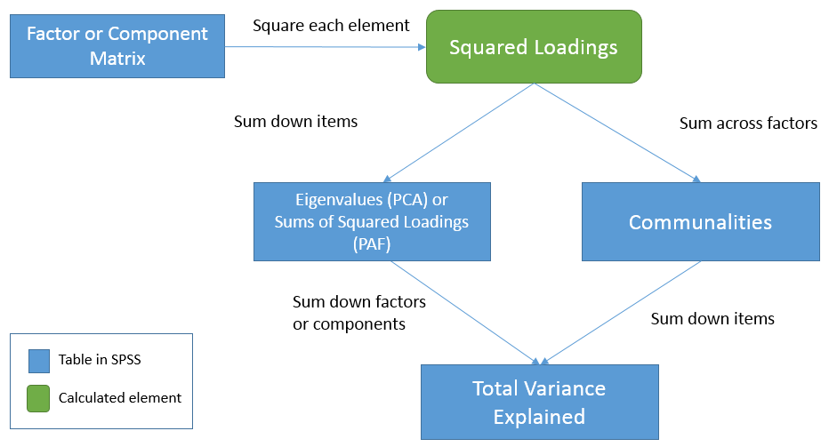
Answers: 1. When there is no unique variance (PCA assumes this whereas common factor analysis does not, so this is in theory and not in practice), 2. F, it uses the initial PCA solution and the eigenvalues assume no unique variance. Factor Matrix (2-factor PAF) Factor Matrixa Item Factor 1 2 1 0.588 -0.303 2 -0.227 0.020 3 -0.557 0.094 4 0.652 -0.189 5 0.560 -0.174 6 0.498 0.247 7 0.771 0.506 8 0.470 -0.124 Extraction Method: Principal Axis Factoring. a. 2 factors extracted. 79 iterations required.First note the annotation that 79 iterations were required. If we had simply used the default 25 iterations in SPSS, we would not have obtained an optimal solution. This is why in practice it’s always good to increase the maximum number of iterations. Now let’s get into the table itself. The elements of the Factor Matrix table are called loadings and represent the correlation of each item with the corresponding factor. Just as in PCA, squaring each loading and summing down the items (rows) gives the total variance explained by each factor. Note that they are no longer called eigenvalues as in PCA. Let’s calculate this for Factor 1: $$(0.588)^2 + 聽(-0.227)^2 + (-0.557)^2 + (0.652)^2 + (0.560)^2 + (0.498)^2 + (0.771)^2 + (0.470)^2 = 2.51$$ This number matches the first row under the Extraction column of the Total Variance Explained table. We can repeat this for Factor 2 and get matching results for the second row. Additionally, we can get the communality estimates by summing the squared loadings across the factors (columns) for each item. For example, for Item 1: $$(0.588)^2 + 聽(-0.303)^2 = 0.437$$ Note that these results match the value of the Communalities table for Item 1 under the Extraction column. This means that the sum of squared loadings across factors represents the communality estimates for each item. The relationship between the three tablesTo see the relationships among the three tables let’s first start from the Factor Matrix (or Component Matrix in PCA). We will use the term factor to represent components in PCA as well. These elements represent the correlation of the item with each factor. Now, square each element to obtain squared loadings or the proportion of variance explained by each factor for each item. Summing the squared loadings across factors you get the proportion of variance explained by all factors in the model. This is known as common variance or communality, hence the result is the Communalities table. Going back to the Factor Matrix, if you square the loadings and sum down the items you get Sums of Squared Loadings (in PAF) or eigenvalues (in PCA) for each factor. These now become elements of the Total Variance Explained table. Summing down the rows (i.e., summing down the factors) under the Extraction column we get \(2.511 + 0.499 = 3.01\) or the total (common) variance explained. In words, this is the total (common) variance explained by the two factor solution for all eight items. Equivalently, since the Communalities table represents the total common variance explained by both factors for each item, summing down the items in the Communalities table also gives you the total (common) variance explained, in this case $$ (0.437)^2 + (0.052)^2 + (0.319)^2 + (0.460)^2 + (0.344)^2 + (0.309)^2 + (0.851)^2 + (0.236)^2 = 3.01$$ which is the same result we obtained from the Total Variance Explained table. Here is a table that that may help clarify what we’ve talked about:
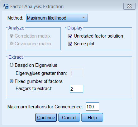
In summary: Squaring the elements in the Factor Matrix gives you the squared loadings Summing the squared loadings of the Factor Matrix across the factors gives you the communality estimates for each item in the Extraction column of the Communalities table. Summing the squared loadings of the Factor Matrix down the items gives you the Sums of Squared Loadings (PAF) or eigenvalue (PCA) for each factor across all items. Summing the eigenvalues or Sums of Squared Loadings in the Total Variance Explained table gives you the total common variance explained. Summing down all items of the Communalities table is the same as summing the eigenvalues or Sums of Squared Loadings down all factors under the Extraction column of the Total Variance Explained table. QuizTrue or False (the following assumes a two-factor Principal Axis Factor solution with 8 items) The elements of the Factor Matrix represent correlations of each item with a factor. Each squared element of Item 1 in the Factor Matrix represents the communality. Summing the squared elements of the Factor Matrix down all 8 items within Factor 1 equals the first Sums of Squared Loading under the Extraction column of Total Variance Explained table. Summing down all 8 items in the Extraction column of the Communalities table gives us the total common variance explained by both factors. The total common variance explained is obtained by summing all Sums of Squared Loadings of the Initial column of the Total Variance Explained table The total Sums of Squared Loadings in the Extraction column under the Total Variance Explained table represents the total variance which consists of total common variance plus unique variance. In common factor analysis, the sum of squared loadings is the eigenvalue.Answers: 1. T, 2. F, the sum of the squared elements across both factors, 3. T, 4. T, 5. F, sum all eigenvalues from the Extraction column of the Total Variance Explained table, 6. F, the total Sums of Squared Loadings represents only the total common variance excluding unique variance, 7. F, eigenvalues are only applicable for PCA. Maximum Likelihood Estimation (2-factor ML)Since this is a non-technical introduction to factor analysis, we won’t go into detail about the differences between Principal Axis Factoring (PAF) and Maximum Likelihood (ML). The main concept to know is that ML also assumes a common factor analysis using the \(R^2\) to obtain initial estimates of the communalities, but uses a different iterative process to obtain the extraction solution. To run a factor analysis using maximum likelihood estimation under Analyze – Dimension Reduction – Factor – Extraction – Method choose Maximum Likelihood.
Although the initial communalities are the same between PAF and ML, the final extraction loadings will be different, which means you will have different Communalities, Total Variance Explained, and Factor Matrix tables (although Initial columns will overlap). The other main difference is that you will obtain a Goodness-of-fit Test table, which gives you a absolute test of model fit. Non-significant values suggest a good fitting model. Here the p-value is less than 0.05 so we reject the two-factor model. Goodness-of-fit Test Chi-Square df Sig. 198.617 13 0.000In practice, you would obtain chi-square values for multiple factor analysis runs, which we tabulate below from 1 to 8 factors. The table shows the number of factors extracted (or attempted to extract) as well as the chi-square, degrees of freedom, p-value and iterations needed to converge. Note that as you increase the number of factors, the chi-square value and degrees of freedom decreases but the iterations needed and p-value increases. Practically, you want to make sure the number of iterations you specify exceeds the iterations needed. Additionally, NS means no solution and N/A means not applicable. In SPSS, no solution is obtained when you run 5 to 7 factors because the degrees of freedom is negative (which cannot happen). For the eight factor solution, it is not even applicable in SPSS because it will spew out a warning that “You cannot request as many factors as variables with any extraction method except PC. The number of factors will be reduced by one.” This means that if you try to extract an eight factor solution for the SAQ-8, it will default back to the 7 factor solution. Now that we understand the table, let’s see if we can find the threshold at which the absolute fit indicates a good fitting model. It looks like here that the p-value becomes non-significant at a 3 factor solution. Note that differs from the eigenvalues greater than 1 criteria which chose 2 factors and using Percent of Variance explained you would choose 4-5 factors. We talk to the Principal Investigator and at this point, we still prefer the two-factor solution. Note that there is no “right” answer in picking the best factor model, only what makes sense for your theory. We will talk about interpreting the factor loadings when we talk about factor rotation to further guide us in choosing the correct number of factors. Number of Factors Chi-square Df p-value Iterations needed 1 553.08 20 |
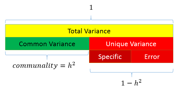 The total variance is made up to common variance and unique variance, and unique variance is composed of specific and error variance. If the total variance is 1, then the communality is \(h^2\) and the unique variance is \(1-h^2\). Let’s take a look at how the partition of variance applies to the SAQ-8 factor model.
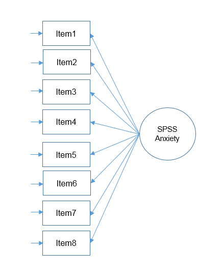
 Here you see that SPSS Anxiety makes up the common variance for all eight items, but within each item there is specific variance and error variance. Take the example of Item 7 “Computers are useful only for playing games”. Although SPSS Anxiety explain some of this variance, there may be systematic factors such as technophobia and non-systemic factors that can’t be explained by either SPSS anxiety or technophbia, such as getting a speeding ticket right before coming to the survey center (error of meaurement). Now that we understand partitioning of variance we can move on to performing our first factor analysis. In fact, the assumptions we make about variance partitioning affects which analysis we run.
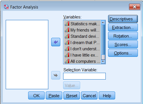
【本文地址】
今日新闻 |
推荐新闻 |